R Studio Conference 2019
This is a notebook summarizing what I learned at the R Studio Conference 2019 Links to all the talks and slide decks,including talks on how to use R in production at scale are available at https://github.com/kbroman/RStudioConf2019Slides
Make sure the libraries being used in each section are installed.
Reproducible Examples with reprex
The reprex package allows you to create a minimal reproducible example that you can share if you are reporting an issue on Github or asking a question on stack overflow. Running the code chunk below after uncommenting will create a new web page with the code and the results that can be shared with others.
# reprex({
#   x <- 1:4
#   y <- 2:5
#   x + y
# })
Categorical data in R
Factor variables in R can be idiosyncratic
x <- c(20,20,10,40,20)
cat(x)
## 20 20 10 40 20
Converting this to a factor variable produces the following
xf <- factor(x)
xf
## [1] 20 20 10 40 20
## Levels: 10 20 40
Converting this factor back to numeric produces the following odd result
x <- as.numeric(xf)
x
## [1] 2 2 1 3 2
The right way to carry out this conversion is as follows
x <- as.numeric(as.character(xf))
x
## [1] 20 20 10 40 20
One also needs to be careful while re-ordering the levels of a factor
ratings1<-  as.factor(c(rep('High',30),rep('Low',10),rep('Medium',20)))
ratings2 <- ratings1
ratings3 <- ratings1
table(ratings1)
## ratings1
##   High    Low Medium
##     30     10     20
cat('Levels: \n')
## Levels:
cat(levels(ratings1))
## High Low Medium
We might want to change the levels of this variable to be Low,Medium,High
The next couple of approaches do not yield expected results.
levels(ratings1) <- levels(ratings1)[c(2,1,3)]
table(ratings1)
## ratings1
##    Low   High Medium
##     30     10     20
levels(ratings2) <- c('Low','Medium','High')
table(ratings2)
## ratings2
##    Low Medium   High
##     30     10     20
The correct approach here would be as follows
ratings3 <- factor(ratings3,levels=c('Low','Medium','High'))
table(ratings3)
## ratings3
##    Low Medium   High
##     10     20     30
The forcats package by Hadley Wickham makes working with factors much more straightforward.
library(forcats)
ratings1<-  as.factor(c(rep('High',30),rep('Low',10),rep('Medium',20)))
ratings1 <- fct_relevel(ratings1,c('Low','Medium','High'))
table(ratings1)
## ratings1
##    Low Medium   High
##     10     20     30
Recoding the levels of the factors are also straightforward.
ratings1 <- fct_recode(ratings1,Poor='Low',Fair ='Medium',Good = 'High')
table(ratings1)
## ratings1
## Poor Fair Good
##   10   20   30
Plenty of other useful functions are available in the forcats package.
Defensive Coding
The testthat and assertthat packages allows us to code defensively. This is typically best practice in software engineering and makes debugging much easier.
For instance if a function is designed to accept a scalar (i.e. a vector of length 1), you may want the function to throw an error if a vector is passed into the function, so that you can adjust the function appropriately.
library(assertthat)

is_odd <- function(x) {
  assert_that(is.numeric(x), length(x) == 1)
  x %% 2 == 1
}


print(is_odd(3))
## [1] TRUE
print(is_odd(2))
## [1] FALSE
#is_odd(c(1,4)) ##Throws an error##
The see_if function returns a logical value and an error message as an attribute that allows execution to continue.
x <- c(1,2)
y <- 'a'
see_if(is.numeric(x), length(x) == 1)
## [1] FALSE
## attr(,"msg")
## [1] "length(x) not equal to 1"
see_if(is.numeric(y), length(y) == 1)
## [1] FALSE
## attr(,"msg")
## [1] "y is not a numeric or integer vector"
The testthat package provides functionality that is essential to software testing. This is useful if you are building packages or writing code that is meant to be used in production
library(testthat)

#Check for equality within numerical tolerance
expect_that(10,equals(10+1e-7))
###Check for exact equality - Throws an error
#expect_that(2*5, is_identical_to(10 + 1e-7))
model <- lm(mpg~wt,data=mtcars)
expect_that(model,is_a("lm"))
###Throws an error
#expect_that(model,is_a("glm"))
If you are making a function you can use this to ensure that it produces warnings when expected.
#  Two functions below pass
expect_that(log(-1), gives_warning())
expect_that(log(-1),
gives_warning("NaNs produced"))

# This one fails if run
#expect_that(log(0), gives_warning())
New Features in R Studio 1.2
R Studio 1.2 allows incorporation of SQL, Python , RCPP, Stan etc seamlessly into your workflow. The reticulate package allows you to use Python within R Studio.
Python
Note the bit below requires R Studio 1.2 and python’s Anaconda installation. Also you might encounter the issue described here and will have to fix by adding the appropriate path to the environment variable
library(reticulate)
use_condaenv("r-reticulate")
import os
os.environ['QT_QPA_PLATFORM_PLUGIN_PATH'] = 'C:/Users/learningmachine/AppData/Local/Continuum/anaconda3/Library/plugins/platforms'
import numpy as np
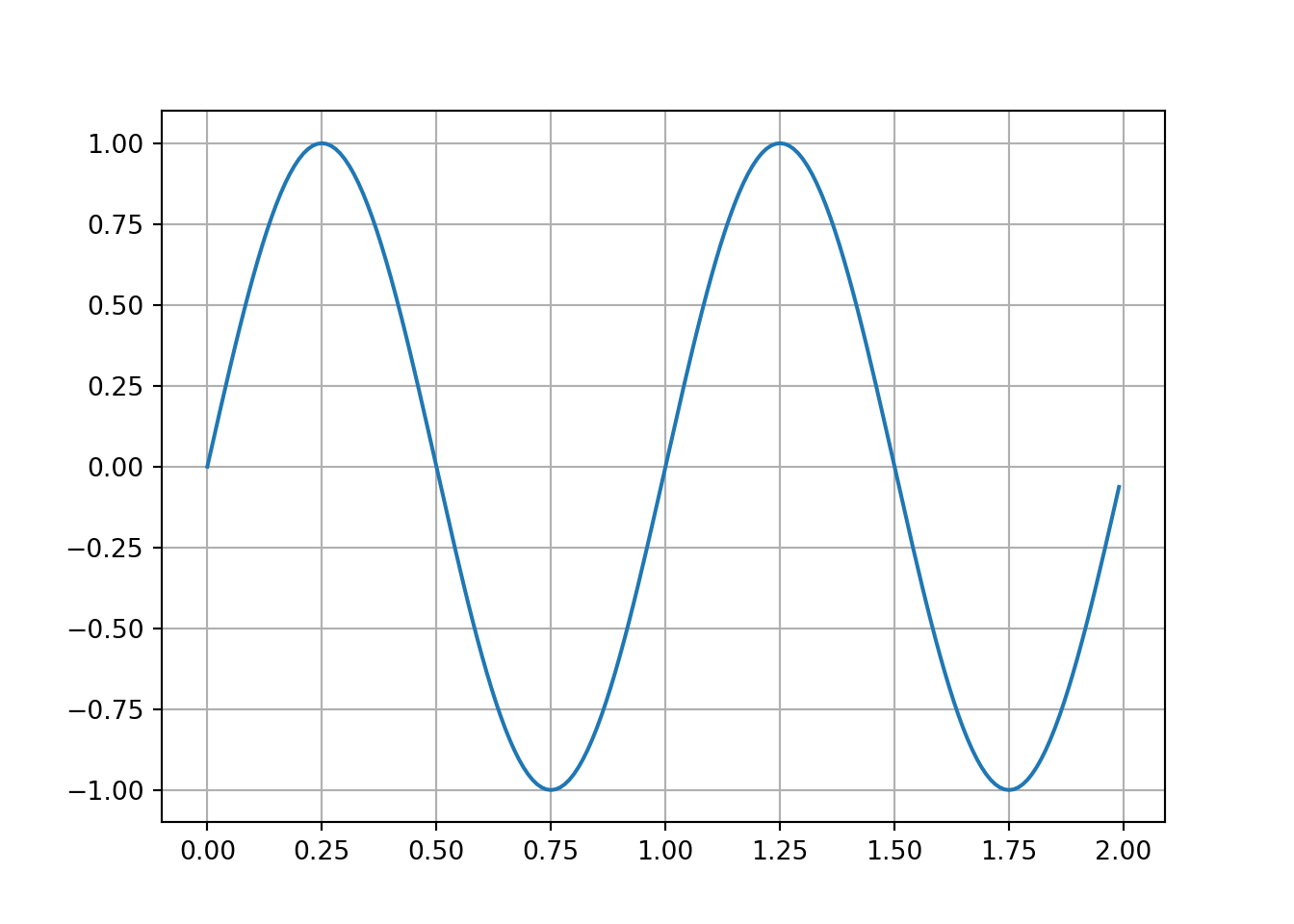
import matplotlib.pyplot as plt
import pandas as pd
x = np.arange(0.0,2,0.01)
y = np.sin(2* np.pi*x)
plt.plot(x,y)
plt.grid(True)
plt.show()
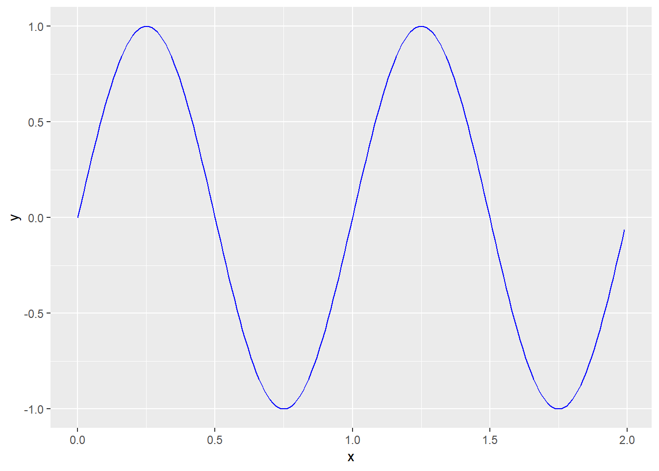
data = pd.DataFrame({'x':x,'y':y})
A pandas dataframe can also be used within R.
library(ggplot2)
ggplot(py$data,aes(x,y))+ geom_line(col='blue')
 SImilarly you can embed SQL or Stan code chunks in your markdown document.
Parsnip - A tidy model interface
library(parsnip)
library(tidymodels)
library(glmnet)
library(randomForest)
Parsnip is tidy version of the popular caret package being developed by Max Kuhn (who also developed caret).This package creates a unified interface to models, organizes them by model type (e.g. Logistic regression, splines etc)and generalizes how to fit them.
First create a model specification
## Linear Regression Model Specification (regression)
##
## Main Arguments:
##   penalty = 0.01
The computation engine can be one of lm, glmnet,stan,spark or keras. Parsnip can translate this general syntax to the model’s argument.
reg_model %>%
  set_engine("glmnet")%>%
    translate()
## Linear Regression Model Specification (regression)
##
## Main Arguments:
##   penalty = 0.01
##
## Computational engine: glmnet
##
## Model fit template:
## glmnet::glmnet(x = missing_arg(), y = missing_arg(), weights = missing_arg(),
##     lambda = 0.01, family = "gaussian")
Note that data is not required for the model specification. Further although glmnet requires the predictors and target to be provided as X,y matrices , parsnip allows you to use a formula.
reg_model %>%
  set_engine("glmnet")%>%
    fit(mpg ~ .,data = mtcars)
## parsnip model object
##
##
## Call:  glmnet::glmnet(x = as.matrix(x), y = y, family = "gaussian",      lambda = ~0.01)
##
##      Df   %Dev Lambda
## [1,] 10 0.8687   0.01
The whole sequence of steps from specification to prediction can be done as follows
linear_reg(penalty =0.01) %>%
  set_engine("glmnet") %>%
    fit(mpg~.,dat =mtcars %>% slice(1:29)) %>% # train set
      predict(new_data = mtcars %>% slice(30:32)) #test set
## # A tibble: 3 x 1
##   .pred
##   <dbl>
## 1  17.9
## 2  10.9
## 3  25.6
If we want to fit the model using multiple penalty values:
preds <-
  linear_reg() %>%
    set_engine("glmnet")%>%
      fit(mpg ~. , data = mtcars %>% slice(1:29))%>%
        multi_predict(new_data = mtcars %>% slice(30:32))


print(preds)
## # A tibble: 3 x 1
##   .pred
##   <list>
## 1 <tibble [80 x 2]>
## 2 <tibble [80 x 2]>
## 3 <tibble [80 x 2]>
This produces a list of dataframes where each list contains predictions for all penalty values considered. To obtain the first 5 predictions for the second data point:
preds %>% pull(.pred) %>% pluck(2) %>% slice(1:5)
## # A tibble: 5 x 2
##   penalty .pred
##     <dbl> <dbl>
## 1 0.00346  10.9
## 2 0.00380  10.9
## 3 0.00417  10.9
## 4 0.00457  10.9
## 5 0.00502  10.9
In the cases of models like random forest where certain data dependent parameters like mtry need to be specified,the model can be specified as follows:
mod <- rand_forest(trees= 1000, mtry =floor(.preds() * 0.75)) %>%
        set_engine("randomForest")

mod %>% translate()
## Random Forest Model Specification (unknown)
##
## Main Arguments:
##   mtry = floor(.preds() * 0.75)
##   trees = 1000
##
## Computational engine: randomForest
##
## Model fit template:
## randomForest::randomForest(x = missing_arg(), y = missing_arg(),
##     mtry = floor(.preds() * 0.75), ntree = 1000)
Fit the model.
mod %>% fit(mpg ~ ., data = mtcars)
## parsnip model object
##
##
## Call:
##  randomForest(x = as.data.frame(x), y = y, ntree = ~1000, mtry = ~floor(.preds() *      0.75))
##                Type of random forest: regression
##                      Number of trees: 1000
## No. of variables tried at each split: 7
##
##           Mean of squared residuals: 5.352952
##                     % Var explained: 84.79
As you can see, the number of predictors used is 75 % of the number of predictors in the data.
floor((ncol(mtcars) - 1) *0.75)
## [1] 7
Time Series in Tidyverse
Tidy and Transform the data using the tsibble package and perform modelling/forecasting using fable. tsibble is a time series version of a tibble/dataframe.
library(tidyr)
library(tsibble)
library(lubridate)
We can use the EuStockMarkets data available in base R which is a ts object.
data("EuStockMarkets")
as_tibble can easily convert this into a tsibble in a long format. Here the index represents time and key identifies the variable that defines the series. Here each stock index ha a unique time stamp.
eu_ts <- as_tsibble(EuStockMarkets)
print(eu_ts)
## # A tsibble: 7,440 x 3 [1s] <UTC>
## # Key:       key [4]
##    index               key   value
##    <dttm>              <chr> <dbl>
##  1 1991-07-01 02:18:28 DAX   1629.
##  2 1991-07-02 12:00:00 DAX   1614.
##  3 1991-07-03 21:41:32 DAX   1607.
##  4 1991-07-05 07:23:05 DAX   1621.
##  5 1991-07-06 17:04:37 DAX   1618.
##  6 1991-07-08 02:46:09 DAX   1611.
##  7 1991-07-09 12:27:42 DAX   1631.
##  8 1991-07-10 22:09:14 DAX   1640.
##  9 1991-07-12 07:50:46 DAX   1635.
## 10 1991-07-13 17:32:18 DAX   1646.
## # ... with 7,430 more rows
Given the index in seconds, the tsibble expects an entry for each second, so the index should be converted to day.
eu_ts2 <-  eu_ts %>%
            mutate(index = as.Date(index))
print(eu_ts2)
## # A tsibble: 7,440 x 3 [1s]
## # Key:       key [4]
##    index      key   value
##    <date>     <chr> <dbl>
##  1 1991-07-01 DAX   1629.
##  2 1991-07-02 DAX   1614.
##  3 1991-07-03 DAX   1607.
##  4 1991-07-05 DAX   1621.
##  5 1991-07-06 DAX   1618.
##  6 1991-07-08 DAX   1611.
##  7 1991-07-09 DAX   1631.
##  8 1991-07-10 DAX   1640.
##  9 1991-07-12 DAX   1635.
## 10 1991-07-13 DAX   1646.
## # ... with 7,430 more rows
One can also calculate the average price of a week or month as follows.
eu_ts %>%
    index_by(Month = floor_date(index,'month'))%>%
        group_by(key)%>%
            summarize(Price =  mean(value))%>% head()
## # A tsibble: 6 x 3 [?] <UTC>
## # Key:       key [1]
##   key   Month               Price
##   <chr> <dttm>              <dbl>
## 1 CAC   1991-07-01 00:00:00 1753.
## 2 CAC   1991-08-01 00:00:00 1800.
## 3 CAC   1991-09-01 00:00:00 1871.
## 4 CAC   1991-10-01 00:00:00 1851.
## 5 CAC   1991-11-01 00:00:00 1814.
## 6 CAC   1991-12-01 00:00:00 1693.
We can also check if there are gaps in the time series as follows.
has_gaps(eu_ts2)
## # A tibble: 4 x 2
##   key   .gaps
##   <chr> <lgl>
## 1 CAC   TRUE
## 2 DAX   TRUE
## 3 FTSE  TRUE
## 4 SMI   TRUE
You can get a 30 day rolling average of the process as follows. Note that the first 29 observations of the rolling mean will be NA.
eu_ts3 <-  eu_ts2 %>%
            group_by(key) %>%
              mutate(avg_30day = slide_dbl(value,~mean(.,na.rm = TRUE),.size=30))

print(eu_ts3 %>% filter_index("1991-08-01"~"1991-09-01") )
## # A tsibble: 88 x 4 [1D]
## # Key:       key [4]
## # Groups:    key [4]
##    index      key   value avg_30day
##    <date>     <chr> <dbl>     <dbl>
##  1 1991-08-02 DAX   1620.       NA
##  2 1991-08-03 DAX   1620.       NA
##  3 1991-08-05 DAX   1623.       NA
##  4 1991-08-06 DAX   1614.       NA
##  5 1991-08-08 DAX   1632.       NA
##  6 1991-08-09 DAX   1630.       NA
##  7 1991-08-10 DAX   1633.     1624.
##  8 1991-08-12 DAX   1627.     1624.
##  9 1991-08-13 DAX   1650.     1625.
## 10 1991-08-15 DAX   1650.     1627.
## # ... with 78 more rows
Tsibble works well with ggplot2.
library(ggplot2)
ggplot(eu_ts2,aes(x=index,y=value)) + geom_line()+
  facet_wrap(.~key,ncol=1)

Forecasting can be done using the fable package which is a tidy implementation of the classic forecast package by Rob Hyndman. This package is being developed by Hyndman’s student Earo Wang and is currently not available on CRAN
Model representation using Broom
Use tidy() to summarize information about models Use glance() to report goodness of fit metrics Use augment() to add information about observations
Produces outputs in a simple tibble
The code below shows what we typically get when building a model
attach(mtcars)
library(broom)
ols_fit <- lm(hp~ mpg + cyl, mtcars)
summary(ols_fit)
##
## Call:
## lm(formula = hp ~ mpg + cyl, data = mtcars)
##
## Residuals:
##    Min     1Q Median     3Q    Max
## -53.72 -22.18 -10.13  14.47 130.73
##
## Coefficients:
##             Estimate Std. Error t value Pr(>|t|)
## (Intercept)   54.067     86.093   0.628  0.53492
## mpg           -2.775      2.177  -1.275  0.21253
## cyl           23.979      7.346   3.264  0.00281 **
## ---
## Signif. codes:  0 '***' 0.001 '**' 0.01 '*' 0.05 '.' 0.1 ' ' 1
##
## Residual standard error: 38.22 on 29 degrees of freedom
## Multiple R-squared:  0.7093,	Adjusted R-squared:  0.6892
## F-statistic: 35.37 on 2 and 29 DF,  p-value: 1.663e-08
Using tidy from the broom package we get:
tidy(ols_fit)
## # A tibble: 3 x 5
##   term        estimate std.error statistic p.value
##   <chr>          <dbl>     <dbl>     <dbl>   <dbl>
## 1 (Intercept)    54.1      86.1      0.628 0.535
## 2 mpg            -2.77      2.18    -1.27  0.213
## 3 cyl            24.0       7.35     3.26  0.00281
Using glance
glance(ols_fit)
## # A tibble: 1 x 11
##   r.squared adj.r.squared sigma statistic p.value    df logLik   AIC   BIC
##       <dbl>         <dbl> <dbl>     <dbl>   <dbl> <int>  <dbl> <dbl> <dbl>
## 1     0.709         0.689  38.2      35.4 1.66e-8     3  -160.  329.  335.
## # ... with 2 more variables: deviance <dbl>, df.residual <int>
Using augment gives information about each observation in the training data
augment(ols_fit)
## # A tibble: 32 x 11
##    .rownames    hp   mpg   cyl .fitted .se.fit .resid   .hat .sigma .cooksd
##    <chr>     <dbl> <dbl> <dbl>   <dbl>   <dbl>  <dbl>  <dbl>  <dbl>   <dbl>
##  1 Mazda RX4   110  21       6   140.     6.84 -29.7  0.0320   38.5 0.00687
##  2 Mazda RX~   110  21       6   140.     6.84 -29.7  0.0320   38.5 0.00687
##  3 Datsun 7~    93  22.8     4    86.7   13.3    6.28 0.121    38.9 0.00141
##  4 Hornet 4~   110  21.4     6   139.     7.00 -28.6  0.0335   38.5 0.00668
##  5 Hornet S~   175  18.7     8   194.    12.8  -19.0  0.112    38.7 0.0117
##  6 Valiant     105  18.1     6   148.     8.75 -42.7  0.0524   38.0 0.0243
##  7 Duster 3~   245  14.3     8   206.     9.79  38.8  0.0656   38.2 0.0258
##  8 Merc 240D    62  24.4     4    82.3   11.6  -20.3  0.0924   38.7 0.0105
##  9 Merc 230     95  22.8     4    86.7   13.3    8.28 0.121    38.9 0.00246
## 10 Merc 280    123  19.2     6   145.     7.47 -21.7  0.0382   38.7 0.00443
## # ... with 22 more rows, and 1 more variable: .std.resid <dbl>
To compare multiple models on goodness of fit:
library(purrr)

fits <- list( fit1 = lm(hp~cyl,mtcars),
              fit2 = lm(hp ~ cyl +mpg, mtcars),
              fit3 = lm(hp~. , mtcars))

map_df(fits,glance,.id = "model") %>% arrange(AIC)
## # A tibble: 3 x 12
##   model r.squared adj.r.squared sigma statistic p.value    df logLik   AIC   BIC
##   <chr>     <dbl>         <dbl> <dbl>     <dbl>   <dbl> <int>  <dbl> <dbl> <dbl>
## 1 fit3      0.903         0.857  26.0      19.5 1.90e-8    11  -143.  310.  327.
## 2 fit1      0.693         0.683  38.6      67.7 3.48e-9     2  -161.  329.  333.
## 3 fit2      0.709         0.689  38.2      35.4 1.66e-8     3  -160.  329.  335.
## # ... with 2 more variables: deviance <dbl>, df.residual <int>
A more realistic application for broom are cases where you want to bootstrap the parameter estimates of a model
Consider the model $$ mpg = \frac{k}{wt} + b + \epsilon, \sim Normal(0,\sigma^2) $$
To estimate the bootstrapped estimates, you can do the following
library(rsample)
boots <- bootstraps(mtcars,times=100)
Function to fit non linear least squares
fit_nls_on_bootstrap <- function(split) {
  nls(
    mpg ~ k/wt + b,
    analysis(split),
    start = list(k=1,b=0)
  )
}
Bootstrap as follows:
boot_fits <- boots %>%
              mutate(fit = map(splits,fit_nls_on_bootstrap),
                     coef_info = map(fit,tidy))

head(boot_fits)
## # A tibble: 6 x 4
##   splits          id           fit       coef_info
## * <list>          <chr>        <list>    <list>
## 1 <split [32/13]> Bootstrap001 <S3: nls> <tibble [2 x 5]>
## 2 <split [32/12]> Bootstrap002 <S3: nls> <tibble [2 x 5]>
## 3 <split [32/11]> Bootstrap003 <S3: nls> <tibble [2 x 5]>
## 4 <split [32/13]> Bootstrap004 <S3: nls> <tibble [2 x 5]>
## 5 <split [32/11]> Bootstrap005 <S3: nls> <tibble [2 x 5]>
## 6 <split [32/11]> Bootstrap006 <S3: nls> <tibble [2 x 5]>
Get bootstrapped coefficients
library(resample)
##
## Attaching package: 'resample'
## The following object is masked from 'package:broom':
##
##     bootstrap
library(tidyr)

data("mtcars")
mtcars_bs <- bootstraps(mtcars,times=20)
boot_coefs <- boot_fits %>%
                unnest(coef_info)

head(boot_coefs)
## # A tibble: 6 x 6
##   id           term  estimate std.error statistic  p.value
##   <chr>        <chr>    <dbl>     <dbl>     <dbl>    <dbl>
## 1 Bootstrap001 k        41.2       3.38     12.2  3.86e-13
## 2 Bootstrap001 b         5.56      1.23      4.53 8.86e- 5
## 3 Bootstrap002 k        38.8       2.82     13.8  1.66e-14
## 4 Bootstrap002 b         6.52      1.03      6.36 5.15e- 7
## 5 Bootstrap003 k        51.7       4.80     10.8  8.12e-12
## 6 Bootstrap003 b         2.61      1.70      1.53 1.36e- 1
Plot bootstrapped estimates as follows
p <- ggplot(boot_coefs,aes(estimate))+
      geom_histogram(binwidth = 2) + facet_wrap(~ term,scales='free')+
        labs(title = "Sampling distribution of k and b",
             y = "Count",
             x = "Value" )


p

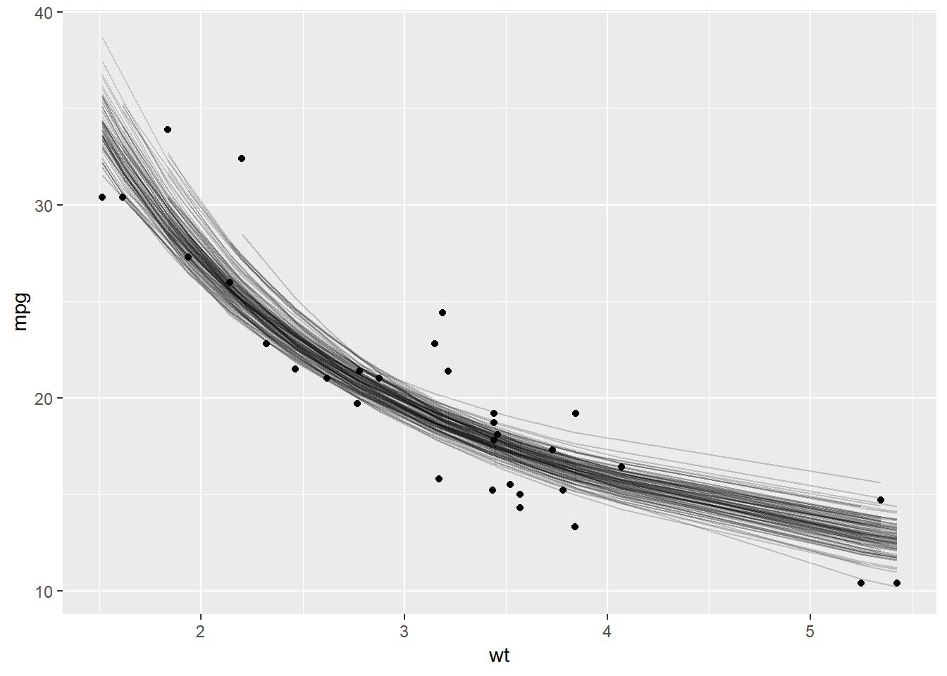
We can also plot the bootstrapped predictions as follows
boot_aug <- boot_fits %>%
              mutate(augmented = map(fit,augment))%>%
                unnest(augmented)


ggplot(boot_aug,aes(wt,mpg))+
  geom_point()+
    geom_line(aes(y = .fitted,group =id),alpha =0.2)
gganimate
Package for animated graphics which extends ggplot2. Additional dependencies will have to be installed.
library(gapminder)
library(gganimate)


ggplot(gapminder, aes(gdpPercap, lifeExp, size = pop, colour = country)) +
  geom_point(alpha = 0.7, show.legend = FALSE) +
  scale_colour_manual(values = country_colors) +
  scale_size(range = c(2, 12)) +
  scale_x_log10() +
  # Here comes the gganimate specific bits
  labs(title = 'Year: {frame_time}', x = 'GDP per capita', y = 'life expectancy') +
  transition_time(year) +
  ease_aes('linear')

Hypothetical Outcome Plots
Hypothetical outcome plots provide an alternative way to visualize uncertainty by animating a finite set of individual draws rather than producing a static representation of distributions.
Load required packages.
library(rsample)
library(purrr)
library(ggplot2)
library(gganimate)
library(transformr)
The plot below uses bootstrapped samples to visualize uncertainty in the trend line.
attach(mtcars)


#Draw bootstrap samples

mtcars_bs <- bootstraps(mtcars,times=20)

mtcars_bs_df <- map_df(mtcars_bs$splits, function(x){
                        return(as.data.frame(x))
                        })

mtcars_bs_df$id <- rep(c(1:20),each=nrow(mtcars))


mtcars %>%
  ggplot(aes(disp,mpg))+
    geom_point()+
      geom_smooth(
        data = mtcars_bs_df,
        aes(group =id),
        se = FALSE,
        alpha = 0.6
      )
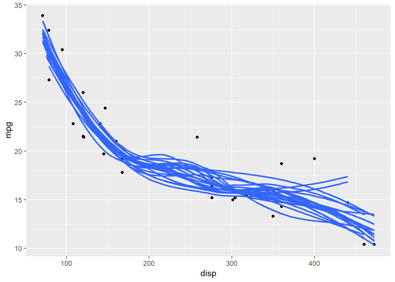
The same can be represented using a hypothetical outcome plot as follows
mtcars_bs_df %>%
  ggplot(aes(disp,mpg))+
    geom_smooth(aes(group =id),se=FALSE,alpha=0.6)+
      geom_point(data=mtcars)+
        transition_states(id)

Datapasta
If you want to quickly copy some sample data from excel or SQL into R, you often have to convert it into csv or excel file and then import it or type it manually. Datapasta is an R Studio add in that provides a much easier alternative.
After installing the package ‘datapasta’ , simply copy the table from an excel file, go to add ins and select the appropriate option.
Here, I simply copied a table from excel using ‘Ctrl+C’ and then selected ‘Paste as data.frame’ from the add ins dropdown.
data.frame(stringsAsFactors=FALSE,
        Name = c("A", "B", "C", "D", "E"),
       Marks = c(87L, 35L, 76L, 34L, 86L)
)
##   Name Marks
## 1    A    87
## 2    B    35
## 3    C    76
## 4    D    34
## 5    E    86
vctrs
This is another package from Hadley Wickham designed to make sure that outputs from functions are predictable.
Sometimes, R does not behave predictable. For instance when combining two factors..
c(factor("a"),factor("b"))
## [1] 1 1
Also..
today <- as.Date('2019-02-23')
tomorrow <- as.POSIXct("2019-02-23 12:00",tz = "America/Chicago")

c(today,tomorrow)
## [1] "2019-02-23" "4248312-08-21"
Also..
c(NULL,tomorrow)
## [1] 1550944800
The vctrs package formalizes the relationships between various datatypes and requires the user to be more explicit when combining different datatypes.
To summarize: Logical –> Integer –> Double Date –> Date-time Factor –>Character Ordered –> Character
library(vctrs)
##
## Attaching package: 'vctrs'
## The following object is masked from 'package:lubridate':
##
##     new_duration
When coercing to character , it is stricter than base R. vec_c below would throw an error
c(1.5,"a")
## [1] "1.5" "a"
#vec_c(1.5,"a")
Instead you have to be explicit..
vec_c(1.5,"x",.ptype = character())
## [1] "1.5" "x"
Unlike in base R, the following works..
vec_c(factor("a"),factor("b"))
## [1] a b
## Levels: a b
Note the order affects the levels..
vec_c(factor("b"),factor("a"))
## [1] b a
## Levels: b a
Similarly when concatenating a factor and an ordered factor…
c(factor("a"),ordered("b"))
## [1] 1 1
The first call below would throw an error..
#vec_c(factor("a"),ordered("b"))
vec_c(factor("a"),ordered("b"),.ptype = character())
## [1] "a" "b"
The date problem does not occur here..
vec_c(today,tomorrow)
## [1] "2019-02-23 00:00:00 CST" "2019-02-23 12:00:00 CST"
Disparate datatypes can be combined into a list
vec_c(today,factor("a"),.ptype=list())
## [[1]]
## [1] "2019-02-23"
##
## [[2]]
## [1] a
## Levels: a
Tidy Evaluation
A tool for metaprogramming. This becomes important when you do not know the names of an object in advance and you want to build a tidyverse pipeline which operates on such objects. This is often the case when you have to operate on user inputs, say in a shiny application where you have to make indirect references with column names stored in variables or passed as function arguments.
It is tidy evaluation that really allows you to use column names below without using quotes.
attach(starwars)

starwars %>%
  filter(homeworld == "Tatooine")%>%
    arrange(height)%>%
      select(name,ends_with("color"))
## # A tibble: 10 x 4
##    name               hair_color  skin_color eye_color
##    <chr>              <chr>       <chr>      <chr>
##  1 R5-D4              <NA>        white, red red
##  2 Shmi Skywalker     black       fair       brown
##  3 Beru Whitesun lars brown       light      blue
##  4 C-3PO              <NA>        gold       yellow
##  5 Luke Skywalker     blond       fair       blue
##  6 Owen Lars          brown, grey light      blue
##  7 Biggs Darklighter  black       light      brown
##  8 Cliegg Lars        brown       fair       blue
##  9 Anakin Skywalker   blond       fair       blue
## 10 Darth Vader        none        white      yellow
To evaluate an expression, the interpreter searches the environment for name-value bindings. In tidy eval, the expression is modified or the chain of searched environments is modified. This is what allows you to use unquoted variable names and work inside a dataframe. This is also referred to as non-standard evaluation.
Tidy eval can be implemented in the following ways..
- Using ‘…’
attach(mtcars)

measure_hp <- function(df,...){
  df %>%
    group_by(...)%>%
      summarize(avg_hp = mean(hp,na.rm=TRUE))}

measure_hp(mtcars,gear)
## # A tibble: 3 x 2
##    gear avg_hp
##   <dbl>  <dbl>
## 1     3  176.
## 2     4   89.5
## 3     5  196.
- Using enquo and !!(called ‘bang!bang!’ operator)
measure<- function(df,group_var,summary_var){
  group_var <- enquo(group_var) #Effectively quotes the variable
  summary_var <- enquo(summary_var)

  df %>%
    group_by(!!group_var)%>%
      summarize(avg_hp = mean(!!summary_var,na.rm=TRUE))}

measure(mtcars,gear,hp)
## # A tibble: 3 x 2
##    gear avg_hp
##   <dbl>  <dbl>
## 1     3  176.
## 2     4   89.5
## 3     5  196.
If you need to manipulate user input that is passed as character strings,you can do the following..
library(rlang)
group_var <- 'gear'
summary_var <- 'hp'

measure(mtcars,!!rlang::sym(group_var),!!rlang::sym(summary_var))
## # A tibble: 3 x 2
##    gear avg_hp
##   <dbl>  <dbl>
## 1     3  176.
## 2     4   89.5
## 3     5  196.
Action and Selection Verbs
dplyr verbs comes in two flavors - action and selection. select is a selection verb while verbs like mutate,group_by and transmute are action verbs.
Action verbs created new vectors and modify the dataframe.Selection verbs look up the position of the columns in the dataframe and re-organizes the dataframe.
Selection verbs are context aware and know about current variables.
starwars %>% select(c(1:height))
## # A tibble: 87 x 2
##    name               height
##    <chr>               <int>
##  1 Luke Skywalker        172
##  2 C-3PO                 167
##  3 R2-D2                  96
##  4 Darth Vader           202
##  5 Leia Organa           150
##  6 Owen Lars             178
##  7 Beru Whitesun lars    165
##  8 R5-D4                  97
##  9 Biggs Darklighter     183
## 10 Obi-Wan Kenobi        182
## # ... with 77 more rows
starwars %>% select(1:height)
## # A tibble: 87 x 2
##    name               height
##    <chr>               <int>
##  1 Luke Skywalker        172
##  2 C-3PO                 167
##  3 R2-D2                  96
##  4 Darth Vader           202
##  5 Leia Organa           150
##  6 Owen Lars             178
##  7 Beru Whitesun lars    165
##  8 R5-D4                  97
##  9 Biggs Darklighter     183
## 10 Obi-Wan Kenobi        182
## # ... with 77 more rows
starwars %>% select(-1,-height)
## # A tibble: 87 x 11
##     mass hair_color skin_color eye_color birth_year gender homeworld species
##    <dbl> <chr>      <chr>      <chr>          <dbl> <chr>  <chr>     <chr>
##  1    77 blond      fair       blue            19   male   Tatooine  Human
##  2    75 <NA>       gold       yellow         112   <NA>   Tatooine  Droid
##  3    32 <NA>       white, bl~ red             33   <NA>   Naboo     Droid
##  4   136 none       white      yellow          41.9 male   Tatooine  Human
##  5    49 brown      light      brown           19   female Alderaan  Human
##  6   120 brown, gr~ light      blue            52   male   Tatooine  Human
##  7    75 brown      light      blue            47   female Tatooine  Human
##  8    32 <NA>       white, red red             NA   <NA>   Tatooine  Droid
##  9    84 black      light      brown           24   male   Tatooine  Human
## 10    77 auburn, w~ fair       blue-gray       57   male   Stewjon   Human
## # ... with 77 more rows, and 3 more variables: films <list>, vehicles <list>,
## #   starships <list>
You can also use selection helpers as follows..
starwars %>% select(ends_with("color")) %>% head()
## # A tibble: 6 x 3
##   hair_color  skin_color  eye_color
##   <chr>       <chr>       <chr>
## 1 blond       fair        blue
## 2 <NA>        gold        yellow
## 3 <NA>        white, blue red
## 4 none        white       yellow
## 5 brown       light       brown
## 6 brown, grey light       blue
starwars %>% select(dplyr::matches("^[nm]a")) %>% head()
## # A tibble: 6 x 2
##   name            mass
##   <chr>          <dbl>
## 1 Luke Skywalker    77
## 2 C-3PO             75
## 3 R2-D2             32
## 4 Darth Vader      136
## 5 Leia Organa       49
## 6 Owen Lars        120
starwars %>% select(10,everything()) %>% head()
## # A tibble: 6 x 13
##   species name  height  mass hair_color skin_color eye_color birth_year gender
##   <chr>   <chr>  <int> <dbl> <chr>      <chr>      <chr>          <dbl> <chr>
## 1 Human   Luke~    172    77 blond      fair       blue            19   male
## 2 Droid   C-3PO    167    75 <NA>       gold       yellow         112   <NA>
## 3 Droid   R2-D2     96    32 <NA>       white, bl~ red             33   <NA>
## 4 Human   Dart~    202   136 none       white      yellow          41.9 male
## 5 Human   Leia~    150    49 brown      light      brown           19   female
## 6 Human   Owen~    178   120 brown, gr~ light      blue            52   male
## # ... with 4 more variables: homeworld <chr>, films <list>, vehicles <list>,
## #   starships <list>
group_by is an action verb, it does not work with selection helpers. The code below does not work.
#starwars %>% group_by(ends_with"color")
Instead you can use..
starwars %>% group_by_at(vars(ends_with("color"))) %>% summarise(mean_height=mean(height))
## # A tibble: 67 x 4
## # Groups:   hair_color, skin_color [50]
##    hair_color    skin_color       eye_color mean_height
##    <chr>         <chr>            <chr>           <dbl>
##  1 <NA>          gold             yellow            167
##  2 <NA>          green            black             173
##  3 <NA>          green-tan, brown orange            175
##  4 <NA>          white, blue      red                96
##  5 <NA>          white, red       red                97
##  6 auburn        fair             blue              150
##  7 auburn, grey  fair             blue              180
##  8 auburn, white fair             blue-gray         182
##  9 black         blue, grey       yellow            137
## 10 black         brown            brown             171
## # ... with 57 more rows
profviz
profviz can be used to profile your code, identify modules that slow down the program and take corrective action.
library(profvis)
#profvis::profvis(mtcars %>% lm(mpg ~ wt +cyl,.))
Using Spark to scale out your jobs
Spark allows you to leverage compute from mutliple machines by distributing computations across multiple machines. The sparklyr package allows you to leverage the power of Spark through R.
Although we connect to spark running on the local machine below, we can easily connect to a cluster provided by a cloud provider. Make sure Java is installed in a directory which does not have spaces or special characters. This link may also be useful
library(DBI)
library(dplyr)
library(sparklyr)                                   #R Interface to Apache Spark
##
## Attaching package: 'sparklyr'
## The following object is masked from 'package:rlang':
##
##     invoke
## The following object is masked from 'package:purrr':
##
##     invoke
#spark_install()                                    #Install Apache Spark

#Add path to java to environment variables
Sys.setenv(JAVA_HOME = 'C:/Users/learningmachine/Java/jre1.8.0_201')


sc <- spark_connect(master = 'local')               #Connect to local cluster
##Make sure you have the mtcars.csv file in your working directory
cars_tbl <- spark_read_csv(sc,"cars","mtcars.csv")     #Read data into spark

summarize(cars_tbl, n =n())                         #Count records with dplyr
## # Source: spark<?> [?? x 1]
##       n
##   <dbl>
## 1    32
dbGetQuery(sc,"SELECT count(*) FROM cars") # COunt records with DBI
##   count(1)
## 1       32
Perform linear regression
ml_linear_regression(cars_tbl,mpg~wt+cyl)
## Formula: mpg ~ wt + cyl
##
## Coefficients:
## (Intercept)          wt         cyl
##   39.686261   -3.190972   -1.507795
You can also define a pipeline and run it on a spark cluster and save it to disk.
pipeline <- ml_pipeline(sc) %>%                #Define Spark pipleine
              ft_r_formula(mpg~wt + cyl)%>%    #Add formula translation
                ml_linear_regression()         #Add model to pipeline

fitted <- ml_fit(pipeline,cars_tbl)
fitted
## PipelineModel (Transformer) with 2 stages
## <pipeline_d2021587785>
##   Stages
##   |--1 RFormulaModel (Transformer)
##   |    <r_formula_d201fa95296>
##   |     (Parameters -- Column Names)
##   |      features_col: features
##   |      label_col: label
##   |     (Transformer Info)
##   |      formula:  chr "mpg ~ wt + cyl"
##   |--2 LinearRegressionModel (Transformer)
##   |    <linear_regression_d201098f3a>
##   |     (Parameters -- Column Names)
##   |      features_col: features
##   |      label_col: label
##   |      prediction_col: prediction
##   |     (Transformer Info)
##   |      coefficients:  num [1:2] -3.19 -1.51
##   |      intercept:  num 39.7
##   |      num_features:  int 2
##   |      scale:  num 1
#ml_save(fitted,"mtcars_model",overwrite = TRUE)
The sparklyr output of a saved Spark ML Pipeline object is in Scala code, which means that the code can be added to the scheduled Spark ML jobs, and without any dependencies in R.
Shiny
Some resources worth exploring on shiny and included in the link shared at the beginning of the document are
Modules: How to compartmentalize your shiny application into modules for easier maintenance and concurrent development
Reactlog 2.0: Library built in Javascript that allows for easier debugging by visualizing reactive dependencies in the app. Th goto tool for reactivity debugging
Miscellaneous
Sunburst Charts
Pretty cool visualization for representing hierarchical data using concentric circles.
library(sunburstR)
sequences <- read.csv(
  system.file("examples/visit-sequences.csv",package="sunburstR")
  ,header=F
  ,stringsAsFactors = FALSE
)

sunburst(sequences)
rayshader
This is a really cool package. According to the documentation:
rayshader uses a combination of raytracing, spherical texture mapping, lambertian reflectance, and ambient occlusion to produce hillshades of elevation matrices. Includes water detection and layering functions, programmable color palette generation, several built-in textures, 2D and 3D plotting options, and the ability to export 3D maps to a 3D printable format.
Try running the code below to see some really cool 3d visualizations.
library(rayshader)

montereybay %>%
sphere_shade(texture="imhof2") %>%
plot_3d(montereybay, zscale=50, water = TRUE, watercolor="imhof2",
waterlinecolor="white", waterlinealpha=0.5)
Other useful/interesting resources
Best practices for naming files: link
mlflow for tracking ML experiments,sharing and deploying : link
All the risk calculators at http://riskcalc.org/ were built by Cleveland Clinic using Shiny